
This blog guides you in importing, transforming, analyzing, and visualizing data seamlessly within a Lakehouse environment using Notebooks.
Prerequisites
- Fabric capacity or Trial License.
- Launch https://app.fabric.microsoft.com/ and start your free trial with Microsoft Fabric.
Refer Lesson 3 – Getting started with Microsoft Fabric blog post.
Step 1 – Create workspace.
Follow the steps to create a workspace in Microsoft Fabric.
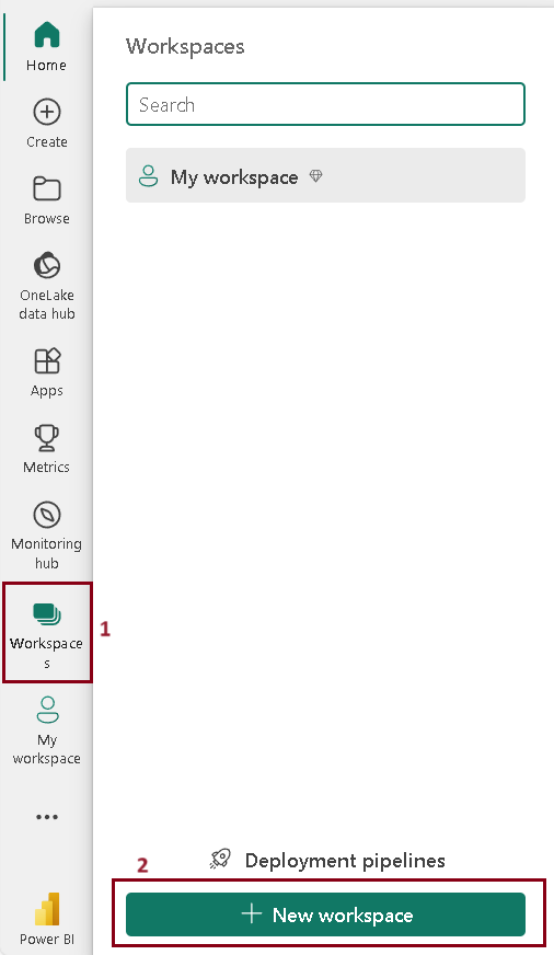
- Sign in to Fabric portal
- Select Workspace (1) –> New Workspace (2)
Take a look at the Lesson – 4 Fabric workspace blog post for more detailed information.
Step 2 – Create Lakehouse
Follow the steps to create lakehouse
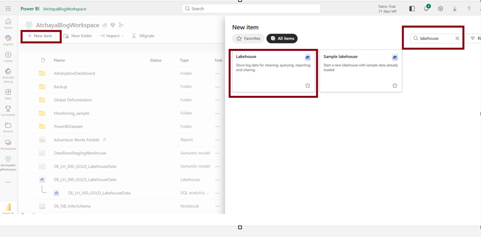
- In the workspace view, click on “New items“.
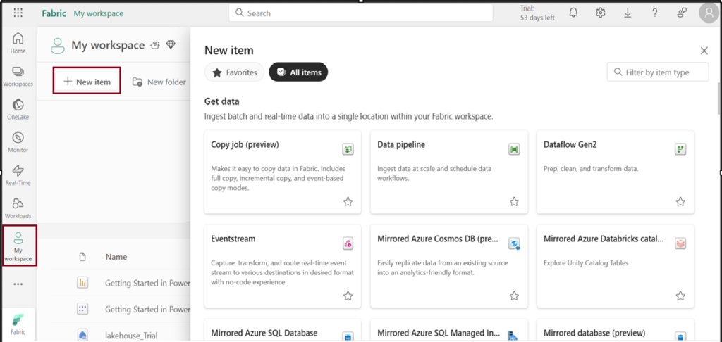
- Choose “Lakehouse ” under the store data option.
- A prompt window will appear; type the desired name for the lakehouse you want to create and click “Create”.
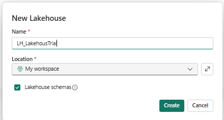
The Lakehouse schemas checkbox is a relatively new Microsoft Fabric feature that was introduced after the early Fabric releases. It allows you to organize your Lakehouse tables into multiple schemas, similar to SQL Server or Azure Synapse.
Without Lakehouse Schemas (older behavior)
- All tables are stored under a single default schema (dbo)
With Lakehouse Schemas Enabled (recommended)
- You can organize tables into logical schemas.
Refer Lesson 7 – Getting started with Microsoft Fabric Lakehouse for detailed information.
Step 3 – Load dataset
Follow the steps to upload the dataset.
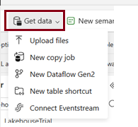
- Once the Lakehouse is created, you will redirect to the lakehouse main page where you can ingest given data. Download the provided datasets locally.
- Download the Olympic dataset CSV file – (taken from Kaggle)
- Upload the files from your local.
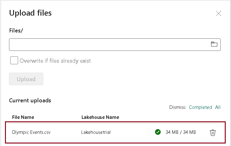
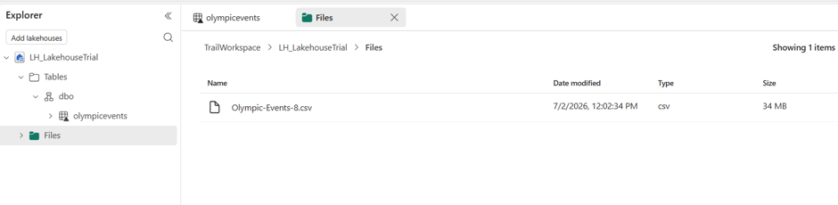
- verify that the CSV files has been uploaded successfully as shown below.
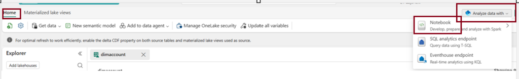
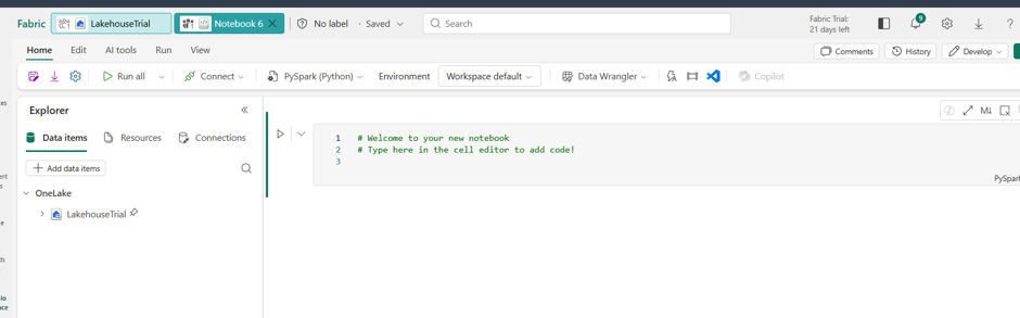
Step 4 – Creating Notebooks
Apache Spark enables data work through interactive notebooks, offering a dynamic environment for code execution and documentation in various languages.
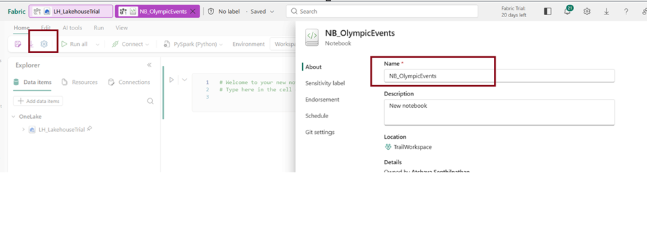
- To Rename the notebook click on settings button and name the notebook and choose the workspace location
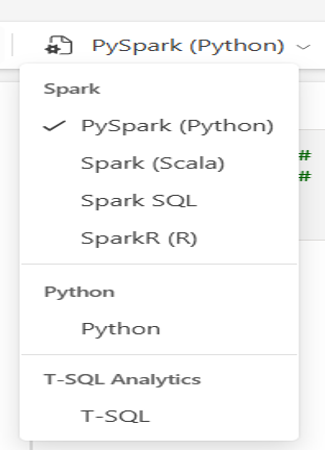
- Spark supports multiple languages. Here I use PySpark since it is one of the commonly used languages on spark and it is default language in Microsoft Fabric notebooks.
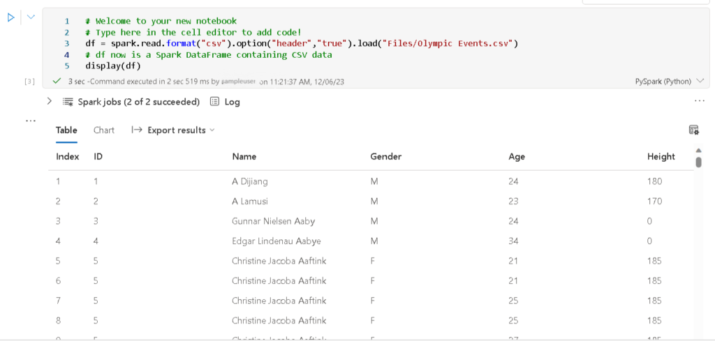
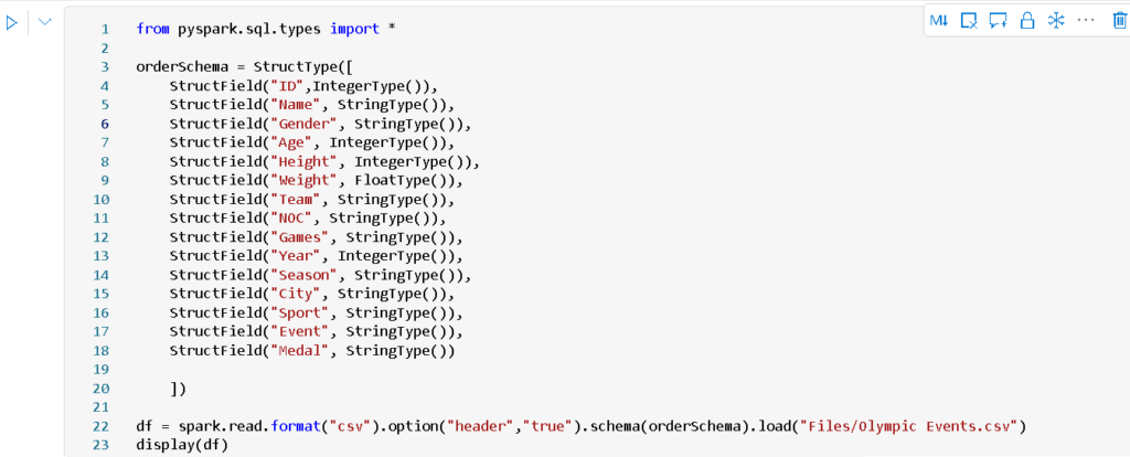
- Add the following code in the cell to load the CSV File into dataframe.

- click ▷ Run cell button on the left of the cell to run the code. When the cell command has complete, review the output. The output shows the rows and columns of data from the Olympic Events.csv
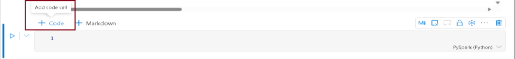
- Click +Code to add new code.
- Revise the code to incorporate schema definition and apply it during the data loading process.
Filer data
- Click +Code icon below the cell output and enter the following code. Run the code and review the results.
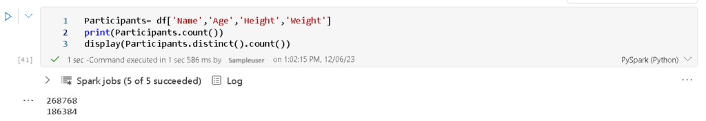
- Participants dataframe is created by selecting specific subset of columns from the df dataframe. Here I selected Name, Age, Height and Weight columns from df and created a new dataframe “Participants”.
- The dataframe [Field1, Field2, ….] syntax is the way of defining subset of columns.
- You can also use Select method to select specific subset of columns.
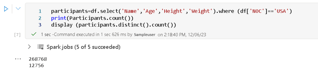
- The above code snippet creates a new DataFrame named ‘participants’ by selecting specific columns (‘Name’, ‘Age’, ‘Height’, ‘Weight’) from the original DataFrame (‘df’). It further filters the data by including only those rows where the ‘NOC’ column equals ‘USA’. In essence, it gathers information about participants from the USA in terms of their name, age, height, and weight.
Group the data
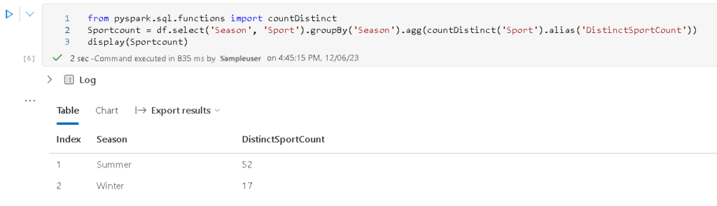
- Click +Code icon below the cell output and enter the following code. Run the code and review the results.
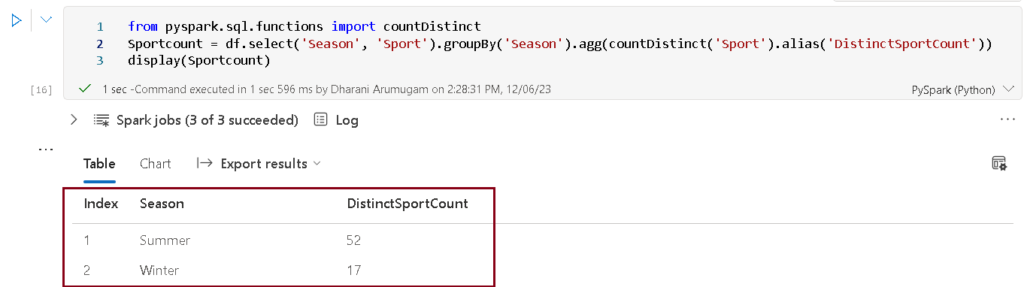
The code uses PySpark to create a DataFrame named ‘Sportcount’ by selecting ‘Season’ and ‘Sport’ columns, grouping the data by ‘Season,’ and calculating the distinct count of sports for each season. The results are displayed, showcasing the unique sport counts for each season in a tabular format.
Step 7 – Transform data
Data engineers often encounter the common responsibility of receiving data in a specific format or structure and then modifying it to facilitate subsequent processing or analysis downstream.
Remove column
- Click +Code icon below the cell output and enter the following code. Run the code and review the results.
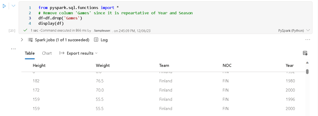
The code employs PySpark to remove the ‘Games’ column from the DataFrame ‘df’ using the ‘drop’ function. This action is taken as the ‘Games’ column is redundant, duplicating information already present in the ‘Year’ and ‘Season’ columns. The updated DataFrame is then displayed using the ‘display’ function.
Reorder columns
- Click +Code icon below the cell output and enter the following code. Run the code and review the results.
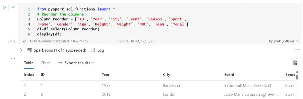
This code rearranges the columns in the DataFrame ‘df’ based on a predefined order specified in the ‘Column_reorder’ list. The resulting DataFrame is then displayed, presenting the updated column arrangement, including ‘ID,’ ‘Year,’ ‘City,’ ‘Event,’ ‘Season,’ ‘Sport,’ ‘Name,’ ‘Gender,’ ‘Age,’ ‘Height,’ ‘Weight,’ ‘NOC,’ ‘Team,’ and ‘Medal.’
Save the transformed data
- Add a new cell with the following code to save the transformed dataframe in Parquet format.
The code writes the PySpark DataFrame (`df`) to a Parquet file format, located in the ‘Files/transformed_data/Olympic’ directory. The “overwrite” mode ensures existing data in the specified directory is replaced, and a confirmation message is printed, indicating the successful saving of the transformed data.
- Run the cell and wait for the confirmation message “Transformed data saved!”. Then in the Explorer pane, Click Refresh under Files folder and select transformed_data folder to verify that it contains a new folder called Olympic.
Step 8 – Visualize data
Follow the steps to visualize the data.
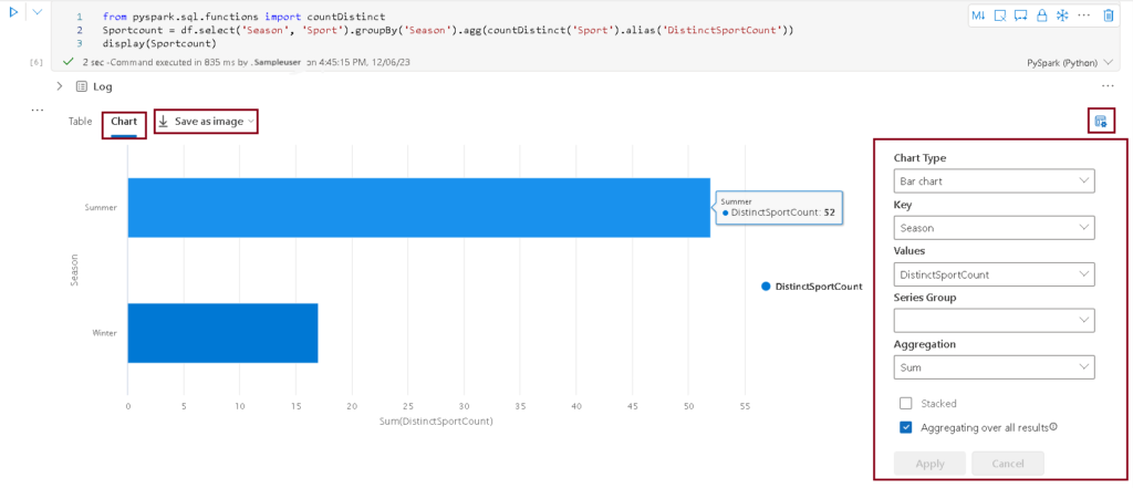
- Add a new cell with the following code and run the cell and observe the results.
- Click on the Chart Tab beneath the cell to display as visual.
- Click on the View option which is at the top right of the chart to display options pane. Set the options as follows and click Apply.
- Chart type – Bar
- Key – Season
- Values – DistinctSportCount
- Series group – blank
- Aggregation – sum
- Stacked – unselected
- Aggregation over all results -selected
- Your chart is displayed as below
- Add a new cell with the following code and run the cell and observe the results.
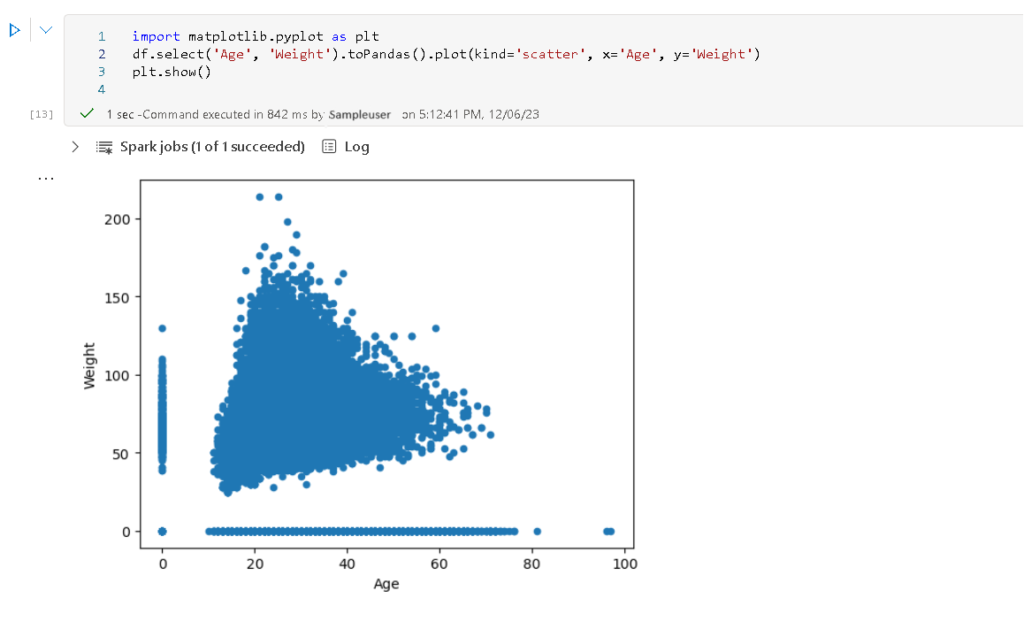
The above code snippet imports Matplotlib, selects the ‘Age’ and ‘Weight’ columns from the PySpark DataFrame (df), converts the selected columns to a Pandas DataFrame, and then creates a scatter plot using Matplotlib. Finally, plt.show() is used to display the scatter plot.
Use seaborn library
While matplotlib allows you to make complex charts, it often requires complex code. Seaborn is built on top of Matplotlib, utilizing its foundation to provide a higher-level and more user-friendly interface for creating attractive statistical visualizations.
- Add a new cell with the following code and run the cell and observe the results.
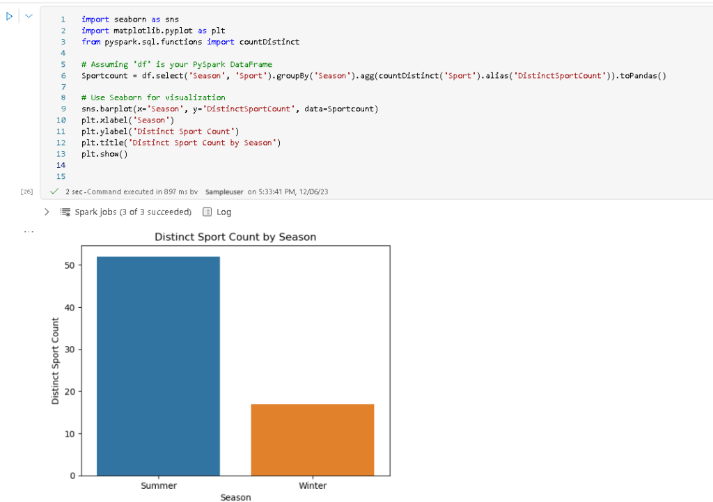
The above code calculates the distinct count of sports by season using PySpark, converts the result to a Pandas DataFrame, and visualizes it with Seaborn using a bar plot.
Step 9 – Working with tables and SQL
The concept of a “data lakehouse” in Spark combines the advantages of a data lake, which allows flexible storage of diverse data, with the structured schema and SQL querying capabilities of a relational data warehouse. In simpler terms, it enables data analysts to use familiar SQL syntax to query and analyse data stored in a more flexible and scalable data lake environment.
Create table
- Add a new code cell to the notebook, and enter the following code, which saves the dataframe of Olympic Events data as a table named olympicdata.
Load the data
A new code cell containing code similar to the following example is added to the notebook.

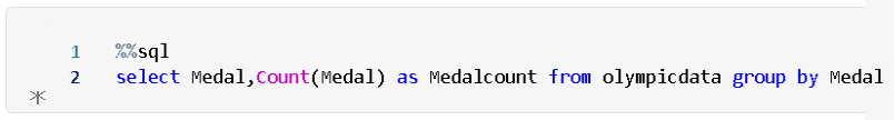
Run SQL query
The “%%sql” is known as a magic command, specifically designed for SQL queries. When you prefix a cell with “%%sql,” it indicates that the content of that cell should be treated as SQL code. This magic command allows you to execute SQL queries directly within the notebook, interacting with a connected database or any environment that supports SQL.
Visualise the data
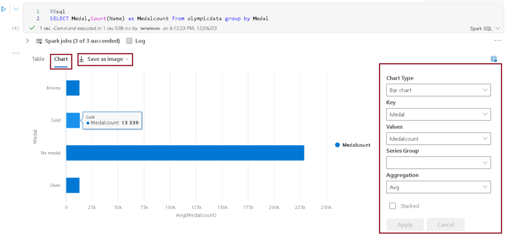
- Add a new code cell to the notebook, and enter the following code. Click Run and observe the results.
- Click on the Chart to view the visual. Click on the View option on the right top corner to display the options pane for the chart.
- You have the option to save the visual by clicking on Save as Image.
Step 10 – Save the Notebook
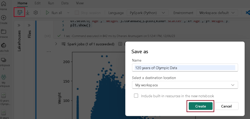
Having completed your data analysis, save the notebook with a descriptive name and conclude the Spark session.
- Click on the Save icon on the menu bar and give the descriptive name to your notebook and click create.
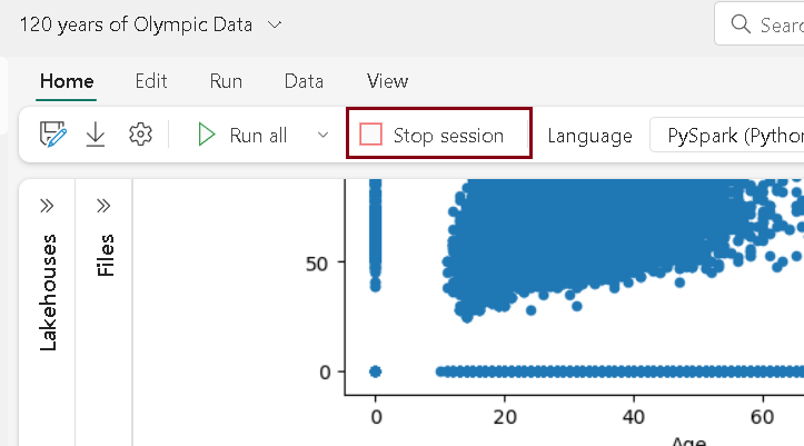
- On the notebook menu, select Stop session to end the Spark session.
| Tags | Microsoft Fabric |
| Useful links | |
| MS Learn Modules | |
Test Your Knowledge |
Quiz |