Lesson 38 – Train Models with Spark Mlib with Microsoft Fabric

This blog guides you through the process of using Apache Spark MLlib with Microsoft Fabric for effective and scalable machine learning. Explore step-by-step instructions to set up your environment and train models seamlessly.

Spark Mlib

Apache Spark MLlib (Machine Learning Library) is a module built on top of the Spark Core that provides machine learning primitives as APIs. It is designed to simplify the development of scalable and distributed machine learning applications on the Apache Spark framework. MLlib offers a wide range of algorithms for common machine learning tasks, making it a powerful tool for handling large datasets and distributed computing environments.

Key features of Spark Mlib

Some of the features of Spark Mlib are

• MLlib supports a variety of machine learning algorithms for classification, regression, clustering, and collaborative filtering.
• MLlib provides tools for feature extraction, transformation, dimensionality reduction, and selection.
• MLlib offers high-level APIs for simplified construction and tuning of machine learning pipelines.
• Seamless integration with Spark components like Spark SQL, Spark Streaming, and GraphX enhances overall functionality.
• MLlib leverages distributed linear algebra and optimization primitives from Spark Core, ensuring scalability.
• Spark MLlib is scalable and user-friendly, suitable for developing efficient big data and machine learning applications.

Prerequisites

• Launch https://app.fabric.microsoft.com/
• Sign in to Microsoft Fabric with your subscription or trial account. Refer Lesson 3 – Getting started with Microsoft Fabric – Pearl Innovations

Steps

• Navigate to the menu bar on the left side and choose “Workspaces” to create new workspace.
• Download the dataset. Taken from CS109 (stanford.edu)

• Create Lakehouse and load the given dataset.
• Click Open notebook ->New notebook to create new notebook.

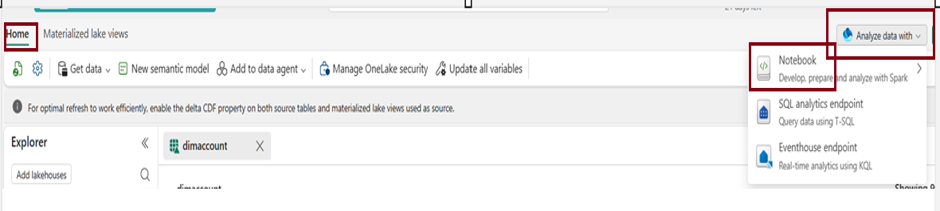
• Within a few seconds, a new notebook will open, comprising a single cell. Notebooks consist of cells that can contain either code or markdown (formatted text).

Set up the environment

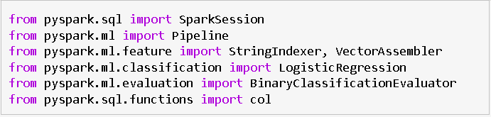
• Various Python libraries and Spark MLlib classes are imported for data analysis and machine learning tasks.

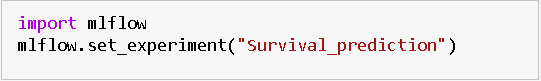
Create Machine Learning Experiment

• Initiate a machine learning experiment using the MLflow API. The mlflow.set_experiment () function will generate a new machine learning experiment in case it doesn’t already exist.

Load Data

• Click on the ellipsis icon next to the desired dataset under “Files,” then select “Load Data” — > “Spark”. It automatically generates Python script.

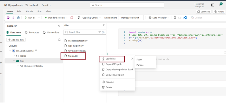
• Click Run to run the script.

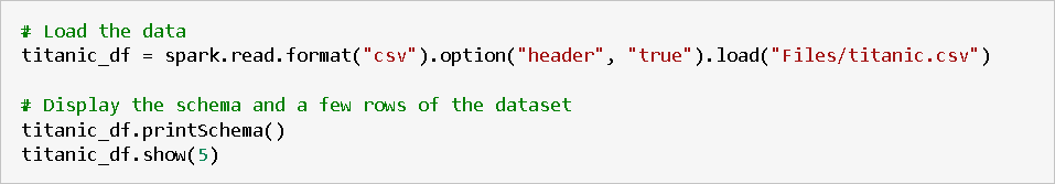
• It prints the schema of the DataFrame and display the first 5 rows to inspect the structure of the data.

Feature Engineering

• Feature engineering involves modifying or creating new features in the dataset to improve the performance of machine learning models.

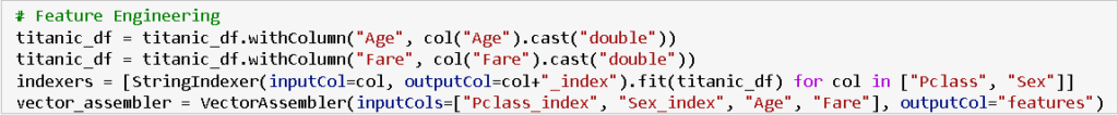
• In this case, the “Age” and “Fare” columns are converted to the double data type, ensuring they are represented as numerical values for better analysis and model training.
• The selected features for the model include indexed representations of categorical variables (e.g., “Pclass_index,” “Sex_index”) and numerical variables (“Age” and “Fare”).
• These features are chosen based on their potential significance in predicting the target variable (“Survived”).

String Indexing and Vector Assembly

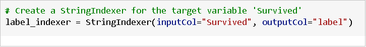
• String indexing is applied to categorical columns (“Pclass” and “Sex”) to convert them into numerical representations.          

• The VectorAssembler then combines these indexed categorical features with numerical features (“Age” and “Fare”) into a single vector column named “features,” which is the input for the machine learning model.

Create Logistic Regression Model

• Logistic Regression is a commonly used algorithm for binary classification problems, such as predicting whether a passenger survived or not in the Titanic dataset (binary outcome – survived or not survived).
• Initialize a Logistic Regression model with specified parameters like maximum iterations, regularization parameters, and elastic net mixing parameter.

• It models the probability of the occurrence of an event using a logistic function. Logistic Regression is interpretable, computationally efficient, and often performs well in classification tasks.

    Create a Pipeline

• A pipeline is used to streamline and automate the machine learning workflow.
• Define a machine learning pipeline with stages for string indexing, vector assembly, and logistic regression model.

• The pipeline enhances code consistency, reproducibility, and modularity, simplifying the deployment and management of end-to-end machine learning workflows in PySpark.

Splitting Data into Training and Testing Sets

• To assess the model’s performance, the dataset is split into two subsets: a training set (70%) used for training the model, and a testing set (30%) used for evaluating the model’s generalization to unseen data.

• The random seed ensures reproducibility of the split.

Train a model

• Training a model involves instructing it to generate predictions from input data, iteratively adjusting internal parameters to minimize prediction errors during the learning process.

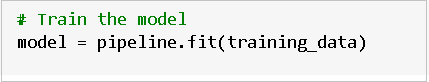
• The line `model = pipeline.fit(training_data)` trains a machine learning model by fitting the defined pipeline to the training data, enabling the model to learn patterns and relationships in the input features.

Making predictions

• Use the trained model to make predictions on the testing set.

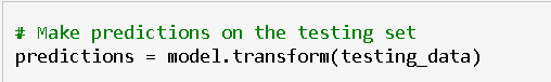
• The above code the trained machine learning model (model) to make predictions on the testing dataset (testing_data).
•  The resulting predictions, including the original features and the model’s predicted labels, are stored in the variable predictions for further evaluation and analysis.

Evaluate the model

• Assessing the model’s performance involves evaluating its accuracy by comparing its predictions to the actual outcomes on a validation or test dataset.

• The code evaluates the model’s binary classification performance on the testing set by computing the area under the ROC curve using the BinaryClassificationEvaluator.

Result

• The calculated area under the Receiver Operating Characteristic (ROC) curve is 0.7623, indicating the model’s performance in distinguishing between positive and negative classes.

• A value closer to 1 indicates a better-performing model in terms of classification accuracy.

Create a visual representation of the prediction

• Generate a visual representation to interpret the model’s outcomes. One effective approach is to construct a ROC curve, providing a comprehensive review of the model’s performance.

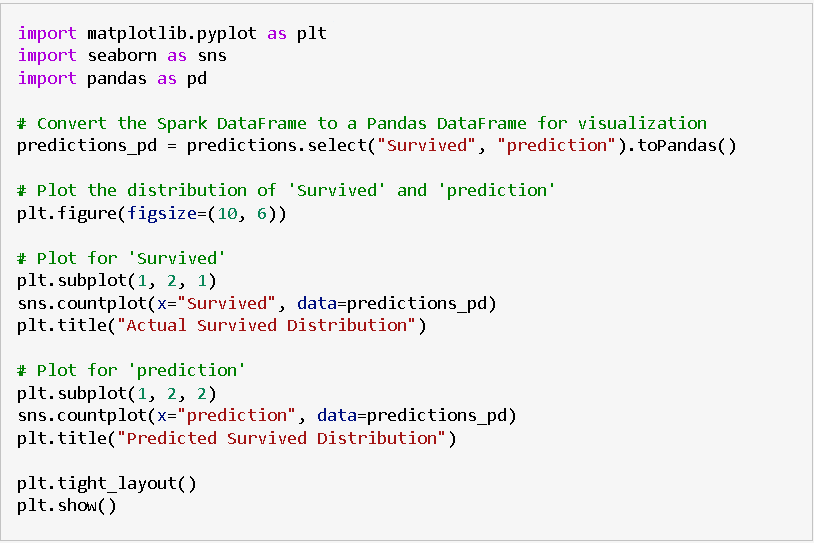
• The provided code uses Matplotlib and Seaborn to create a side-by-side comparison of the distribution of actual survival outcomes and predicted survival outcomes. It involves the following steps:

1. Conversion to Pandas DataFrame
   • The PySpark DataFrame “predictions” containing actual (“Survived”) and predicted (“prediction”) values are converted to a Pandas DataFrame named “predictions_pd” to facilitate visualization.
2. Visualization
   • A figure with two subplots is created using Matplotlib, each representing the distribution of survival outcomes.
   • The left subplot shows the distribution of actual survival outcomes using Seaborn’s countplot.
   • The right subplot displays the distribution of predicted survival outcomes based on the model’s predictions.
   • The visualizations provide a comparative view of how well the model predictions align with the actual survival distribution.
3. Display
   • The plots are displayed using plt.show().

This visualization helps assess the model’s performance by comparing the predicted and actual distributions of survival outcomes in a visually intuitive manner.